Posts

Showing posts with the label GIS 4930 - Special Topics

Lab 5: M2.2 Interpolation

Lab 5: M2.2 Interpolation

Our labs on Surfaces continued on with Lab 5 with Interpolation with Thiessen Polygons, IDW, and Spline. 

Thiessen Polygons - as the name suggests - creates polygons between the sampling points.

IDW (Inverse Distance Weighting) - a DEM that gives weight to its nearest neighbors but can be "spotty".

Spline - DEM that smooths the differences between points. 


Lab 4: M 2.1 TINs and DEMs

Lab 4: M 2.1 TINs and DEMs


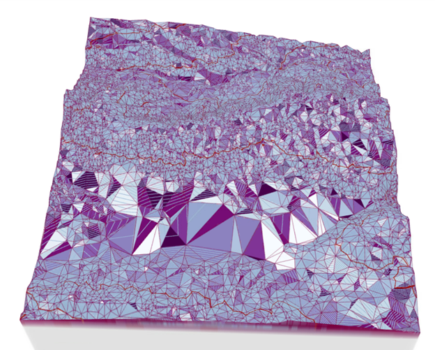
This week we started our labs on Surfaces. The first one being on TINs and DEMs. 

I was familiar with all the tools used from previous labs. 

We explored the difference between the TINs and DEMs elevation models and all their different attributes. One of the main differences between the two is that DEM looks more natural but TINs is more precise. 

It was interesting going through all the renders possible for the TIN layer. Finding the right combination of colors to show the different slopes, edges, and contours so they don't overwhelm each other was a bit of a task. 


Lab 3: M1.3: Assessment

Lab 3: M1.3: Assessment


Our 3rd and final lab in Data Quality was on Assessment. 

We compared the Jackson County road network to the US Census TIGER road network data. 

Before confining the roads to 1 km by 1 km grids for analysis the difference in street length between the two networks was about 576 kilometers, with the TIGER data seeming more complete. 

After clipping the roads to the grids the difference between the two networks rose by approximately 6300 kilometers. 

I then used the Pairwise intersect tool at the suggestion from a classmate. I had to do some trial and error with the summarize tool to get all the required information. There was 1 grid that had zero roads and 1 grid with only TIGER road data. 

I ended up with percentages in the high negatives. The highest being in negative 500 to 1000. A visual inspection shows that the TIGER road data may be roads that were planned and had not been developed yet or trails. I redid things a few times and kept getting the same results. 


Lab 2: M1.2 Standards

Lab 2: M1.2 Standards

Our 2nd lab in GIS4930 builds off skills we learned in the first lab as it pertains to accuracy. 

Since I've been playing catch up from last week, I was able to review the discussion board before starting the lab and take advantage of the various tips that had been posted (mainly the missing orthros and the excel sheet)

Overall no issues with the lab. I manually labeled the three sets to match each other and since the excel sheet already had the formulas, the data entry and analysis were a breeze.

I split the study area up into 4 quadrants and randomly selected from there. A few points had to be moved due to lack of viable streets. I used Calculate Geometry to get the correct points on each set and then copied and pasted into excel from there. 


Albuquerque City

Positional Accuracy: Tested 18.41 feet horizontal accuracy at 95% confidence level.


StreetMap USA

Positional Accuracy: Tested 175.76 feet horizontal accuracy at 95% confidence level.


I passed Security+, so that journey for now has come to an end. Thinking Cloud, Data, or Project for next year though. 

Lab 1: M1.1 Fundamentals

Lab 1: M1.1 Fundamentals


Welcome back blog readers! It's been.. not that long. But we're at the beginning of the end! Its officially the Fall Semester. I am taking 3 courses this semester. Special Topics in Geographic Science, Aerial Photography and Remote Sensing, and the GIS Internship course. 

Since the GIS Internship course runs the whole semester, a few blogs from that course will be scattered through our usual line up. 

But the first blog due is for Special Topics. 

This first week in GIS4930 we went over the Fundamentals of Data Quality, specifically, Calculating Metrics for Spatial Data Quality to better understand the difference between precision and accuracy. 

We learned how to calculate the vertical and horizontal position accuracy and precision, calculate root-mean-square-error (RMSE) and cumulative distribution function (CDF)

The only "new" tool I don't think we have been specifically told to use before was the measure tool, but I use this frequently at work, so no issues. 

Honestly, besides the math, the thing that gave me the most pain was remembering how to edit a chart in excel (which prior blog posts have address our love-hate relationship). 


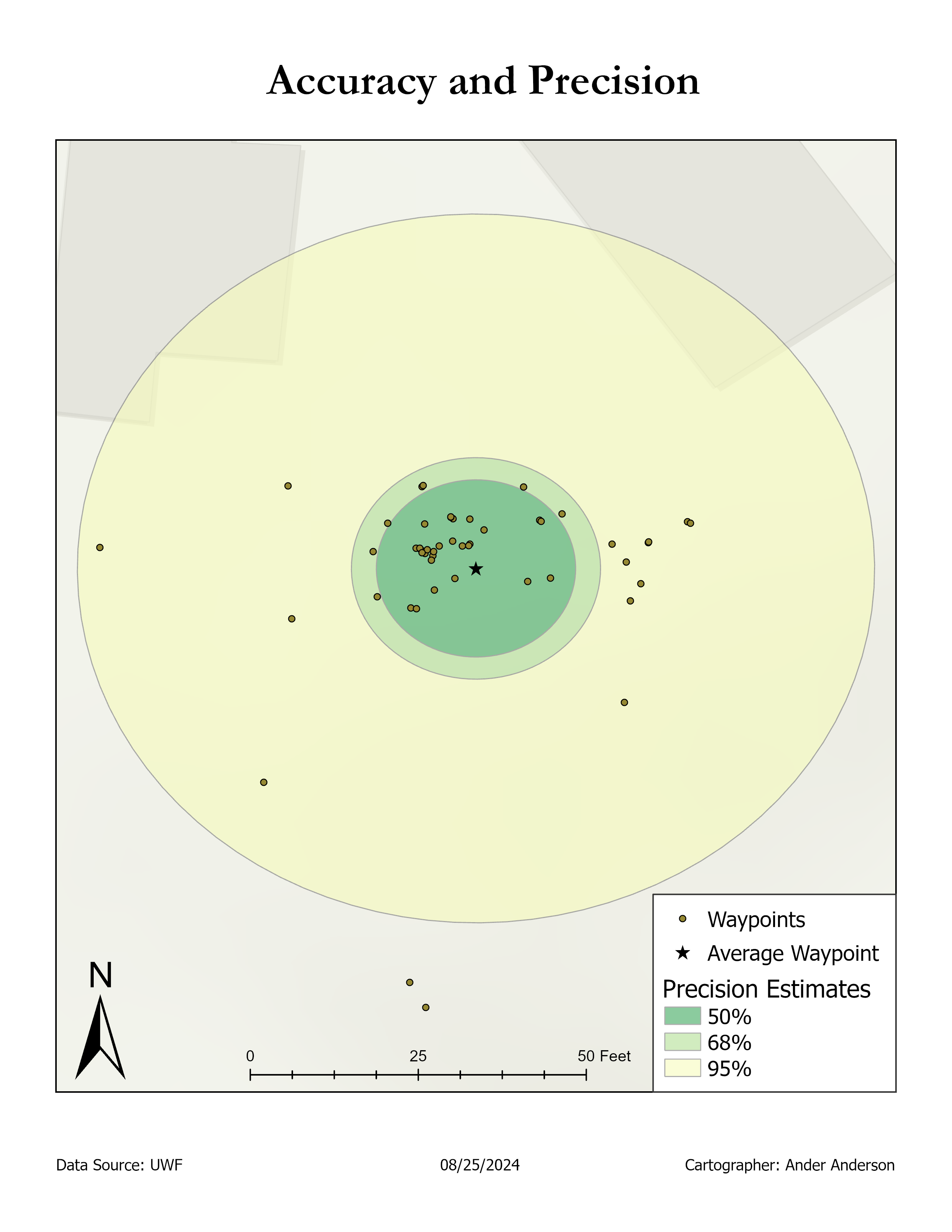
The map below shows the projected waypoints, the average location, and buffers for the precision estimates. 


Horizontal accuracy

-6.066

Horizontal precision

4.293

Difference

10.359


Horizontal accuracy measures how close the GPS measurements are to the true location. Horizontal precision measures the spread of the GPS measurements around the mean location. I believe our lab instructions said it best - The larger the value, the lower the precision. The larger the distance, the lower the accuracy. 


Thankfully this lab was fairly direct. I have been studying for the CompTIA Security+ Exam and I'll be taking it tomorrow (Wednesday) so hopefully my next blog I can report that my CompTIA journey for this year is complete and I can completely focus on GIS again.